Real time space weather prediction with Solar Orbiter

This article was originally written as a Solar Orbiter nugget of science to summarise my Laker et al. 2023 paper

Space weather has the potential to significantly disrupt human technology both in space and on the ground, including loss of satellites, damage to power grids and communication blackouts¹. Fortunately, many of these effects can be mitigated with preventative measures should the arrival time and severity of the storm be known in advance. Since the largest of the geomagnetic storms are driven by coronal mass ejections (CMEs), this makes timely and accurate predictions of CME arrival times and internal structure extremely important.

Unlike many natural hazards, it is relatively straightforward, through continuous monitoring of coronal images, to spot when a large CME has been launched from the Sun. However, simulating the CMEs journey through the solar wind is a more challenging task. Many sophisticated solar wind and CME models still deal with arrival time errors of $\pm 10$ hours, due to uncertain estimates of the CME’s initial parameters² and the complex interaction of the CME with the ambient solar wind that can lead to significant deflections, deformations and rotations^3,4.

Information regarding the orientation of the CME’s magnetic field, a primary indicator of geo-effectiveness, is often as valuable as the predictions of arrival time⁵. Knowing the potential impact of the CME, rather than just its arrival time, can limit the number of false positives and make predictions more useful for those commercial applications where there is a high cost of mitigation, e.g., putting a spacecraft into a safe mode.

Currently, a number of spacecraft (ACE, Wind and DSCOVR) monitor the real time plasma conditions, providing us with a valuable early warning system. However, on a heliospheric scale, these spacecraft are located too close to Earth, at the L1 Lagrange point, only giving us a warning of less than 45 minutes for potential space weather events.

Our understanding of CMEs and the solar wind is now being pushed forward by a new generation of spacecraft sent to investigate the inner heliosphere, including Solar Orbiter along with Parker Solar Probe and even BepiColombo as it makes its way to Mercury. Together, this constellation of spacecraft can give us insights that would not be possible with a single spacecraft⁶. Several authors have used multi-point observations to better understand the complex morphology of CMEs^7,8,9, especially as they interact with the solar wind and other CMEs. In the context of space weather prediction, several case studies have shown how a space weather monitor far further upstream that L1 could be beneficial in predicting the arrival time and geo-effectiveness of CMEs^10,11,12. For instance, Amerstorfer et al. 2018¹² made use of a 2010 CME to show how measurements from the MESSENGER spacecraft could reduce the arrival time error at STEREO-B (located around 1au), which acted as a proxy for Earth.

Now, as recently reported in Laker et al. 2023¹³, Solar Orbiter has been able to replicate these case studies but in real time, acting as a space weather monitor in March 2022. Solar Orbiter’s low latency data products were used to provide real time information about the magnetic field in the solar wind, along with a fortuitous trajectory that crossed the Sun-Earth line in March 2022, allowed the authors to temporarily transform Solar Orbiter into a real time space weather monitor at more than 0.5au from the Earth.

Although originally intended to help point Solar Orbiter’s telescopic arsenal, the low-latency data product is of lower time resolution and quality than the scientific grade data typically released 90 days after download. To overcome these challenges, the Solar Orbiter MAG team¹⁴ created a pipeline to remove over 50 different heater signals and interference from other instruments aboard the spacecraft. The result was a cleaned product that could be available only 12 minutes after it was taken in the solar wind, which includes the 4 minutes it takes for light to travel such a large distance.

As Solar Orbiter crossed the Sun-Earth line, two CMEs were observed by the spacecraft, at the times depicted as red dots in Figure 1. Both case studies were tracked along their journey with the STEREO-A Heliospheric imager (HI) and subsequently measured in situ by Wind at L1.

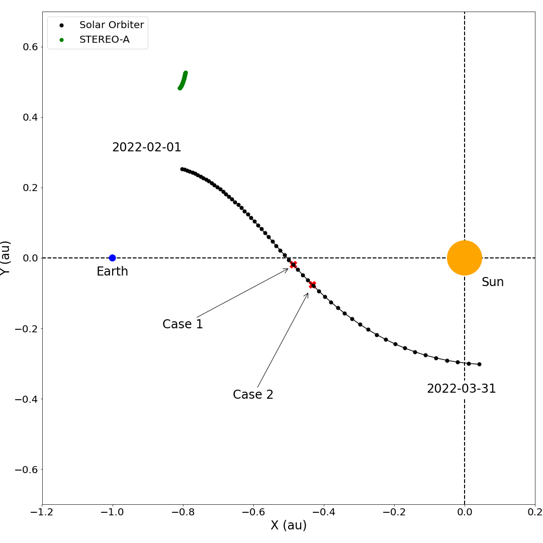Figure 1: Trajectory of Solar Orbiter in the ecliptic plane of the Sun centred GSE frame between 1 February and 31 March 2022. The spacecraft crossed the Sun-Earth line on 6 March and then subsequently measured the two CME events on 7 March and 11 March, respectively. Each point represents the Solar Orbiter position at the start of each day. The Sun is represented by the orange filled circle, the Earth as a blue dot.

Similar to the Amerstorfer et al. 2018¹² study, the authors used data from the upstream spacecraft to constrain the arrival time predictions from the ELEvoHI model. Under normal operation, this model uses an average of 210 ensemble members to estimate the arrival time of a CME at Earth. However, by only keeping those ensemble members that were within $\pm4$ hours of the observed arrival time at Solar Orbiter (red dots in Figure 2), they improved both the accuracy and precision of the model. Specifically, the mean absolute error was reduced from 10.4 to 2.5 hours and 2.7 to 1.1 hours in the two case studies. Therefore, for the first time, a numerical model was constrained with data from 0.5 au to produce an updated prediction before the actual arrival of the CMEs at Earth.

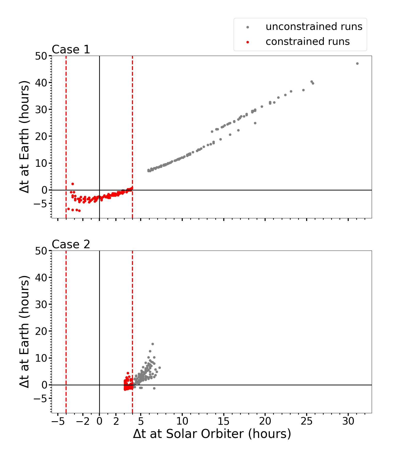Figure 2: Difference between simulated and true arrival time at Solar Orbiter (x axis) and Earth (y axis) for the 210 ensemble member runs from ELEvoHI. By constraining the model with the Solar Orbiter arrival time $\pm4$ hours (red dashed lines), only 99 and 85 ensemble members were kept for the two cases, respectively (red scatter points).

Comparing measurements from Solar Orbiter and Wind, in Figure 3, revealed that the magnetic structure of the CME sheath and flux rope were remarkably similar for the second case study, despite being separated by 0.5 au. Crucially, the magnetic response at Earth (D$_{ST}$ and SYM/H indices) was consistent with the shape of the $B_z$ signature at Solar Orbiter, displaying three dips before the flux rope slowly rotated northward. So, at least for this event, the magnetic storm indicators at Earth were strongly correlated to the magnetic structure seen at 0.5 au around 40 hours prior. While the other case study was a more complex interaction between two CMEs, these results are still encouraging and suggest that a future upstream space weather monitor could not only predict the arrival of a CME, but the sub-structure of the flux rope and sheath region on an hourly time scale.

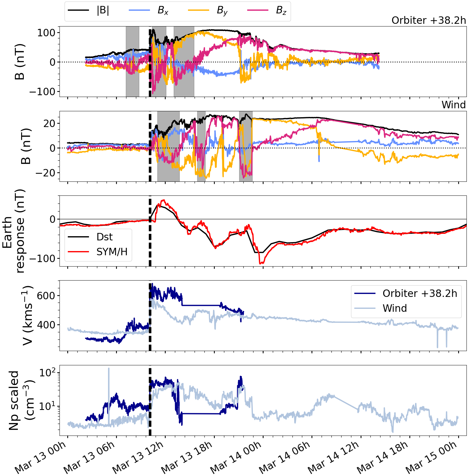Figure 3: In situ measurements for a CME case study in the GSE coordinate system, where vertical dashed lines show the start times of the event. Top panel shows the magnetic field components at Solar Orbiter, which have been shifted by 38.2 hours to match with the shock front at Wind in the panel below. The proton density, $Np$, at Solar Orbiter has been scaled by $1/r^{2}$. Both spacecraft observe three regions of negative $B_z$, followed by a flux rope with a positive $B_z$. This led to a geomagnetic storm at Earth, which also exhibited three dips in the D$_{ST}$ and SYM/H indices.

In future, more models can make use of this data, either to constrain the output or to initiate a CME simulation away from the complex environment near the Sun^3,15. Fortunately, the opportunity to use Solar Orbiter for this purpose repeats once a year. When the next Carrington level event barrels towards Earth, maybe the Solar Orbiter MAG team will be the first to alert the world about its internal structure.